A POST-FLOOD ICE-AGE MODEL CAN ACCOUNT FOR QUATERNARY FEATURES
by Michael J. Oard National Weather Service Great Falls, Montana
WHAT THIS ARTICLE IS ABOUT
A model of an ice age caused by the Genesis flood is summarized. It proposes solutions to a number of ice-age problems. A rough estimate of the time to reach glacial maximum and the melting time is presented. This model can account for the Greenland and Antarctica ice sheets.
INTRODUCTION
Many phenomena that have not yet been adequately explained occurred in the latest period of geologic time. The Pleistocene is part of post-flood time in a creation-flood paradigm. This period was dominated by an ice age at mid and high latitudes. Thus, an adequate ice-age model must be able to explain these phenomena.
One Quaternary puzzle is the widespread evidence for large lakes and rivers in currently arid and semi-mid regions around the world. This is explained as being the result of a wet climate during a pluvial (rainy) period. For example, in the southwestern United States Lake Bonneville was 17 times larger and 285 m deeper than its shriveled remnant, Great Salt Lake. Six times the current runoff likely was needed to maintain Lake Bonneville in a cool ice-age climate (Smith and Street-Perrott 1983).
Another major problem is the extinction of the woolly mammoth in Siberia and Alaska. Many thousands, possibly millions, of them lived in this region, which today is characterized by bitterly cold winters and permafrost which produces massive summer swamps. Little food is available for large herds of mammals. For the mammoths and many other types of mammals to have lived there, it seems likely that the climate was much warmer and without permafrost. A rapid and permanent climatic cooling may have been responsible for the extinction of these animals.
A third important ice-age problem is the widespread evidence of cold-tolerant animals living side by side with warmth-loving animals (Martin and Klein 1984). For example, reindeer fossils have been found with hippopotamus fossils in the Thames River valley of southern England (Grayson 1984, p. 16). Evidently, the hippopotamus ranged into northern England, France, and Germany during early post-flood time (Sutcliffe 1985, p. 24). Then at the end of the ice age, when most scientists believe the climate to have been warming, many large mammals became extinct about five times as many as died out over the combined twenty to thirty presumed previous glaciations.
During deglaciation large river valley meanders were cut by runoff from the melting ice sheets. Water volumes about 60 times the present flow are indicated (Dury 1975). This evidence suggests catastrophic melting.
These and other questions can be solved by a model for a post-flood ice age. Such a model has been proposed (Oard in press, b). A brief summary of this model and an estimate of the duration of the ice age have been published elsewhere (Oard 1979, 1980, 1987). In this article I will summarize the model, giving particular attention to the time required to develop and melt the ice sheets. Throughout I will suggest solutions to ice-age questions.
A POST-FLOOD ICE-AGE MODEL
The requirement for an ice age is a combination of much cooler summers and greater snowfall at mid and high latitudes (Fletcher 1968, p. 93). The snow cover during the first year must last through the summer, and sufficient moisture must be added year by year to continue growth. If summers are very cold, a modest snowfall increase over the average can be adequate; if the summer cooling is small, a many-fold increase would be necessary. This presents a major problem for conventional models of the ice age in that cooler air is less able to hold moisture (Byers 1959, p. 161). The lack of moisture for an ice age is perhaps the reason why more than 60 theories for the ice age have been proposed (Eriksson 1968, p. 68). Nearly all these theories have serious scientific problems, as stated by Charlesworth (1957, II:1532) over 30 years ago:
Pleistocene phenomena have produced an absolute riot of theories ranging 'from the remotely possible to the mutually contradictory and the palpably inadequate.'
This statement was even more true ten years ago, according to John (1979, p. 57), and the currently popular astronomical theory of the ice age is no exception (Oard 1984 a, b, 1985).
Using a computerized energy-balance model, Williams (1979) found that with a snow depth given by twice the present cold-season snowfall, a 10-12ºC average summer temperature drop was required for a perennial snow cover in northeast Canada. The basis for this conclusion is that melting of snow is controlled more by solar radiation, which is abundant at higher latitudes in summer, than by air temperature (Paterson 1981, p. 313). Researchers have been focusing too much on the latter. At the above temperature change, the air would hold 60% less water vapor at saturation. This is a very large decrease in moisture, which was not taken into account by Williams, whose model already slightly overestimated the summer snow cover. It is evident that if a long-age mechanism for summer cooling could be found, the precipitation likely would fall far short of the requirement for an ice age. The need for an adequate cooling mechanism which also provides abundant moisture is one of the main difficulties in developing a successful ice-age model on a conventional time scale. The model presented in this paper proposes that the requirements for an ice age can be met in the climatic upheaval following the Genesis flood.
The flood was a tremendous tectonic and volcanic event. Layers of volcanic ash mixed within sedimentary rocks and large basaltic lava flows attest to extensive flood volcanism. Over 50,000 volcanoes are estimated on land and on the bottom of the ocean. Many of these likely formed during the flood. At the end of the flood a large amount of volcanic dust and aerosols would presumably have been trapped in the upper atmosphere. This would cause strong surface cooling over continental areas by reflecting a significant quantity of solar radiation back to space, while infrared radiation continued to escape. Once a snow cover was established, an increased portion of sunlight would be reflected back to space, reinforcing the cooling. Cooling of the atmosphere above a snow cover is especially effective over barren land, as most land would be immediately after the flood. For instance, a fresh snow cover over barren land will reflect 80% of the sunlight back to space under clear skies, while a snow-covered forest only reflects back 25%. Bare soil under clear skies reflects 10-25% of the sunlight back to space. Greater concentration of atmospheric moisture at higher latitude causes more low cloudiness, which is now known to cool the surface (Ramanathan et al. 1989).
The vast shroud of volcanic dust and aerosols resulting from the flood upheavals would settle out of the atmosphere within a few years, but the planet likely would not settle down to geophysical equilibrium for hundreds of years. Further volcanism at a variable but gradually decreasing rate would be expected, continuing the cool summer temperatures over land. Surficial sediments provide a large amount of evidence for much more ice-age volcanism than there is at present. Charlesworth (1957, II:601-603) states that signs of ice-age volcanism are visible over the whole earth. This evidence is based on numerous ash layers, sometimes covering large areas. In the western United States alone, at least 68 large ash falls have been identified during the ice age (Izett 1981). The ash from one large eruption on New Zealand covered 1×10⁷ km2 of the Southern Hemisphere, and probably blocked out practically all sunlight over the entire earth (Froggatt et al. 1986). Many of the ice-age volcanic eruptions were much larger than those which have occurred over the past 200 years. Modern large eruptions, such as Tambora and Krakatoa, are not even expected to leave an ash layer that would survive conspicuously over large areas (Froggatt et al. 1986). Sulfur aerosols are believed to be the primary long-lasting cause of surface cooling, since volcanic dust can settle and be washed out of the atmosphere in a matter of months. Basalt lava flows, which are less explosive than such eruptions as Tambora and Krakatoa, are now considered to have been a major source of upper atmospheric sulfur aerosols in the past, especially since these milder eruptions contain ten times as much sulfur compounds as do the more explosive eruptions (Devine, Sigurdsson and Davis 1984).
Most scientists do not accept a volcanic cooling mechanism because of their greatly expanded time scale. Since glacial geologists believe each ice age lasted around 100,000 years (Imbrie and Imbrie 1979), volcanism. is seen as an insignificant factor. However, the possibility that high volcanic activity could initiate continental glaciation is acknowledged:
... volcanic explosions would need to be an order of magnitude more numerous than during the past 160 years to result in continental glaciation equivalent to the Wisconsin glacial episode (Damon 1968, p. 109).
The Wisconsin glacial episode is the last glaciation in the standard ice-age chronology. Bray (1976) has suggested that a period of high volcanism may indeed have triggered glaciation by causing cooler summers for a few years, which in turn resulted in an extensive summer snow cover. The snow cover then reinforced the initial cooling, and an ice age was started. Bray (1976) writes: "I suggest here that such a [snow] survival could have resulted from one or several closely spaced massive volcanic ash eruptions."
The water for the flood is assumed to have come predominantly from the "fountains of the great deep" (Genesis 7:11). Enough water was added to the pre-flood oceans to cover all the mountains over the entire planet (Genesis 7:19). Although pre-flood mountains either were much lower than present ones (Psalm 104:5-9) or were lowered by tectonic activity, the added water was still substantial. The "fountains of the deep" imply water shooting high up into the air from cracks or fissures in the earth. This water must have been trapped in the crust of the earth and released under pressure. If we assume that this water came from deeper sources than our usual aquifers, it would be hot water, since the crust warms 30ºC per km of depth. The temperature of subterranean water today varies from the warm temperatures of hot springs to about 350ºC in geothermal vents along the mid-ocean ridges (Kerr 1987). Therefore, the ocean after the flood would be warm. How warm depends upon such variables as the amount and average temperature of the added water and the average temperature of the pre-flood ocean. The post-flood ocean could easily have been hot. But if the average temperature was much warmer than 30ºC, marine life as we know it now would have been seriously threatened. This suggests using 30ºC as a probable maximum temperature for the oceans immediately following the flood. Because the tectonic activity associated with the flood would mix the ocean water, a generally uniform ocean temperature from pole to pole and from the surface to the bottom would have resulted.
Oxygen isotope changes in foraminifera from ocean sediments indicate that the bottom water temperature was relatively warm in the past, compared to the present 4ºC. This evidence comes from pre-Quaternary sediments (Kennett 1982, p. 717). For example, Paleocene ocean bottom temperatures are calculated to have been as warm as 13ºC. Most creationists would consider pre-Quaternary sediments to be flood deposits. This is probably correct for indurated sediments. Unconsolidated ocean sediments are mostly dated by index microfossils, especially foraminifera. Pre-Quaternary microfossils could easily have lived during the ice age. If all biogenic sediments on the ocean floor, except the most recent, were laid down in the waning stages of the Genesis flood and during the ice age, the trend in oxygen isotope changes in pre-Quaternary sediments, even if only crudely valid, would support a warmer ocean bottom at the beginning of the ice age.
The warm post-flood ocean provides the abundant moisture required for the ice age. The cooling mechanisms would have little effect on the ocean temperature until well into the ice age, due to the large heat capacity and circulation of the ocean. Evaporation rate is proportional to the ocean surface temperature. If all other variables remain constant, the evaporation rate at an ocean surface temperature of 30ºC is over three times greater than it is at 10ºC, and over seven times greater than it is at 0ºC. The mid- and high-latitude atmosphere especially would receive much more moisture than today. Evaporation also depends upon how dry and cold the air above the ocean is, and on how fast the wind blows. Consequently, evaporation would be strongest in the storm belt off the east coasts of North America (Bunker 1976) and Asia and off the coast of Antarctica, where cold and relatively dry air blows off the continent and over the warm water in the dry sectors of storms. In the ice-age era, the ocean circulation would continually replenish warm ocean water in these areas. This replacement would come from the deep ocean and from lower latitudes. At this time the Arctic Ocean would be not only ice free, but also quite warm! Large quantities of moisture, as well as heat, would be released into the polar atmosphere.
The average precipitation over mid- and high-latitude continents would have been at least three times the current rate. This factor and the Genesis flood would explain the evidence of a pluvial period in currently arid and semi-arid areas. Large basins, such as those found in the southwestern United States, would have been filled with water at the end of the flood. After the flood, higher precipitation during the ice age would have partially maintained most of these large lakes in currently arid areas and provided adequate moisture for larger streams and rivers. The evidence that a much wetter climate in present-day arid and semi-arid areas occurred after the flood is provided by the existence of large extinct drainage networks in the Sahara Desert and the discovery of remains of such animals as the elephant, hippopotamus, crocodile, giraffe, antelope, and rhinoceros along these now-dry rivers (McCauley et al. 1982, Pachur and Kröpelin 1987).
Many areas which are close to the warm water, such as northern Siberia and Alaska, would have cool summers and mild winters with high precipitation. Warmer ice-age winters for these regions can be surmised from a climate simulation without the Arctic ice cap. Keeping all other variables the same as today, but removing the Arctic ice cap and maintaining the surface temperature at freezing, Newson (1973) discovered winter temperatures would warm 20-40ºC over the Arctic Ocean and 10-20ºC over northern Siberia and Alaska. Precipitation would also have been much heavier than today. Since the Arctic Ocean immediately after the flood would be much warmer than freezing, ice-age temperatures would be significantly warmer than those reported by Newson. As a result of warmer, wetter winters, the woolly mammoth and other cold-tolerant mammals would find a favorable habitat in Siberia and Alaska during the ice age. A warm Arctic Ocean would explain the development of an ice dome in the normally very dry Keewatin area, northwest of Hudson Bay.
The storm tracks of today generally are associated with the strongest upper winds aloft the jet stream which are found in areas of strong horizontal temperature change. The storms and winds aloft are generally parallel to the isotherms with the cold air on the left facing downwind. In today's climate the strong horizontal temperature change is constantly shifting over mid and high latitudes. No one area receives an over-abundance of precipitation. But in the post-flood climate, the cooling mechanisms would operate continually to keep the mid- and high-latitude continents cool. When juxtaposed to warm oceans, these cool continents would cause the greatest temperature difference to remain stationary year-around, lying parallel to the shoreline of mid- and high-latitude continents. Due to the contrast between snow-covered and non-snow-covered land, another belt of large temperature difference would be found at the edge of developing ice sheets.
Westerly winds aloft blowing across the Himalaya and Rocky Mountains would reinforce the stationary thermal pattern over North America (Held 1983). However, this atmospheric phenomenon would tend to shift the major storm track farther offshore from eastern Asia. This factor plus the high mountains of eastern Asia, which would cause significant downslope warming and drying of west winds, and the warmth of the Arctic Ocean is probably the reason why 90% of the Northern Hemisphere ice developed around the Atlantic Ocean (Charlesworth 1957, II:1146). The lowlands of Alaska and eastern Asia were not glaciated another difficulty for modeling based on a long time scale.
The unique meteorological features outlined above would result in the rapid establishment of a snow cover in favorable continental areas. It would be a snowblitz in that the ice age developed simultaneously over large areas (except for strips that were particularly close to warm ocean water). After accumulating to a significant depth, the snow would turn to ice, either by pressure and recrystallization at depth, or from refreezing of meltwater. In the post-flood snowblitz, storms would often develop near the southeastern coast of the United States and move northeastward. These storms would be very much like present-day "northeasters" that wrack the eastern seaboard of the United States and southeast Canada every year. Northeasters cause crippling ice, heavy snow, and gale force winds with a resultant loss of life and more than a billion dollars in property damage each year (Dirks, Kuettner and Moore 1988). In a typical wintertime storm most of the precipitation falls in the colder air portion of the storm with a narrow band of showers along the cold front, south of the low pressure center. In the post-flood climate northeasters would have carried much more water vapor (due to the much warmer ocean), probably extended over a larger area, and developed much more frequently. In areas of great temperature contrast, one to three large storms and several small storms can develop in a week. To illustrate the potential for a snowblitz that turns into an ice age, I will conservatively assume that only one northeaster a week developed and moved up the east coast of North America. Let us assume that each storm dropped 5cm water equivalent of snow over a broad area, which is only twice the amount of snow in modern northeasters. At this rate with no summer runoff, almost 3m of ice would accumulate in a year. In 200 years the depth would reach 580 m over favorable areas of northeastern North America.
At the beginning of the ice age, snow and ice most likely extended well south into the central United States, since volcanic dust is particularly effective for cooling continental interiors. As volcanism diminished, increased penetration of sunshine would melt the ice sheet in the central United States, due to its southerly latitude. The ice margin would retreat to a more or less equilibrium position in the north-central United States. Heavy precipitation would then strongly erode the till left behind in the central United States. Clay, soil, and vegetation would form rapidly. On this basis, after the ice age the central United States would have an "ancient-looking" landscape, with the clay interpreted as the B-horizon of ancient soils.
DISHARMONIOUS ASSOCIATIONS
Northwest Europe would have been dominated by warm onshore winds during the early part of the ice age. Rather warm winters in this area would not have inhibited the hippopotamus and other warmth-loving mammals from migrating as far as northern England. These warmth-loving animals would mix with cold-tolerant animals forced to live south of the ice sheets. As a result the fossil remains of these animals would show a unique mix of seemingly incompatible animals in today's climate. This phenomenon is called disharmonious associations and was common during the ice age. Graham and Lundelius (1984, p. 224) state:
Late Pleistocene communities were characterized by the coexistence of species that today are allopatric [not living in the same geographic area] and presumably ecologically incompatible.... Disharmonious associations have been documented for late Pleistocene floras ..., terrestrial invertebrates ..., lower vertebrates ..., birds ..., and mammals....
To account for hippopotamus fossils so far north it has been postulated that they lived during a warm "interglacial" period. However, we live in a warm interglacial period today, but today's interglacial climate is much too cold for hippopotamuses in northwest Europe. Furthermore, they are often found in the same sediment layer with animals that prefer a cold climate. Grayson (1984, p. 16) states:
In the valley of the Thames [southern England], for instance, woolly mammoth, woolly rhinoceros, musk ox, reindeer (Rangifer tarandus), hippopotamus (Hippopotamus amphibius), and cave lion (Felis leo spelaea) had all been found by 1855 in stratigraphic contexts that seemed to indicate conternporaneity....
To account for disharmonious associations some researchers postulate the mixing of fossils from glacial periods with those from "interglacial" periods. However, the postulated mixing is not a likely explanation for many disharmonious associations, because the associations are widespread and disappear in post-ice-age sediments. Graham and Lundelius (1984, p. 224) write:
Most of the presently available evidence suggests that individual stratigraphic units are deposited in too short a time in relation to the rate of environmental change for this [mixing of remains] to be a likely cause.... The widespread occurrence of disharmonious faunas in Pleistocene deposits also indicates that these associations were much too common to be spurious in all cases. In addition, if these associations are caused by sedimentary mixing, their frequency should be about the same for all time periods; but disharmonious associations are rare in Holocene [post-ice age]faunas, and in stratified faunas they usually disappear at the Pleistocene/Holocene contact.
Disharmonious associations during the ice age do not conform to expectations based on a conventional time scale, but can be explained by a mild post-flood ice age. An ice age in the standard framework is very cold. Computer simulations of the climate at ice-age maximum indicate temperatures on the order of 10ºC colder than today immediately south of the ice sheets (Manabe and Broccoli 1985). The climate was also drier at maximum. A colder, drier climate is also theoretically expected well before maximum glaciation, according to a system based on the conventional time scale. One would not expect warmth-loving, and even many cold-tolerant, animals and plants to survive relatively close to the ice sheets under the above conditions. Severe climatic stress should have occurred. However, great numbers of the animals existed, many of them large (McDonald 1984). Moreover, as the ice sheets melted, presumably from a warming climate that should have been more favorable to survival, many species became extinct the opposite of what one would expect.
THE LENGTH OF TIME
The duration of a post-flood ice age is of special concern to biblical creationists, since the ice age is cited as one example among many to support a long evolutionary time scale. The length of time for an ice age can be divided into two estimates: 1) the time necessary to reach glacial maximum, when the largest volume of ice was locked up into the ice sheets, and 2) the time required to melt the ice sheets (except, of course, for the ones in Antarctica and Greenland).
The time to reach maximum ice volume depends upon the unique controlling conditions. Volcanism would gradually wane with time, but the ice age would still continue if the snow that fell during the warmer half of the year remained fresh with a high reflectivity. This requires heavy snow, which, in turn, depends upon the ocean surface temperature in the precipitation region. In other words, as the ocean cooled, the available moisture would gradually diminish, and a time would come when decreasing snowfall and increasing sunshine would reverse glacial buildup. Therefore, the ocean surface temperature, which is proportional to the average temperature of the deep ocean, controls the length of time taken to reach glacial maximum. The average temperature of the ocean today is 4ºC. The ice-age maximum would certainly occur before the ocean cooled to this temperature. I will assume that the ice-age maximum occurred at a threshold ocean temperature of 10ºC, or a 20ºC drop in temperature from the end of the flood to glacial maximum. This change represents a net heat loss of 3.0×1025 calories, most of which would occur in the form of latent heat of evaporation at mid and high latitudes (Bunker 1976, Budyko 1978).
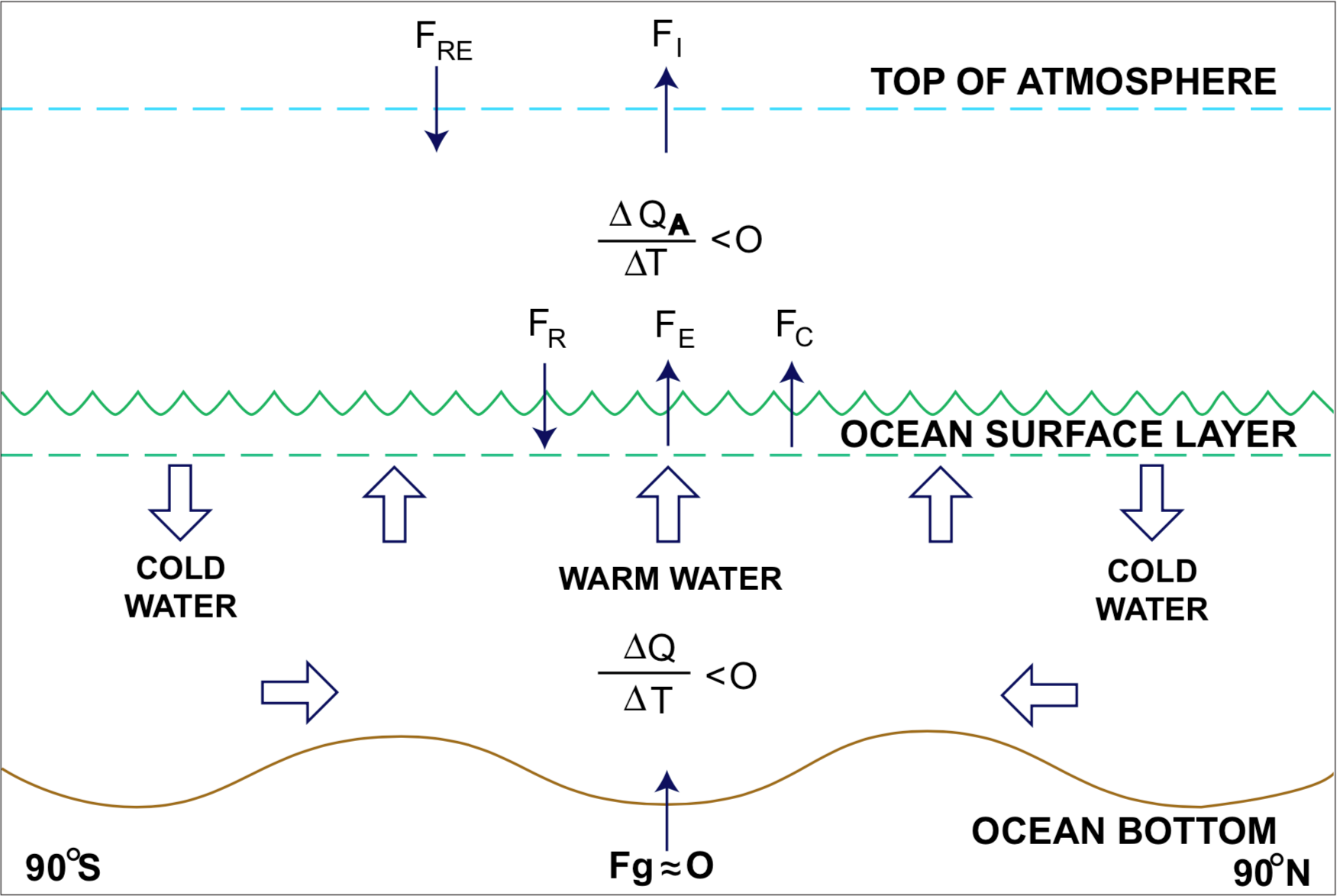
The time to cool the ocean can be estimated from the heat balance equations for the ocean and the atmosphere and from reasonable assumptions of post-flood climatology. These heat balance equations relate the heat input and output to the change in heat content of the ocean and atmosphere. Figure1 illustrates the components of the heat balance. The direction of the arrows indicates the heat flux.
FIGURE 1. Oceanic and atmospheric heat balance. FRE is the net solar radiation absorbed by the earth-atmosphere system, FI is the net infrared radiation escaping from the top of the atmosphere, FR is the net surface radiation, FE is the evaporative heat flux, FC is the conductive heat flux, FG is the geothermal heat, DQ/DT is the cooling rate of the ocean, DQA/DT is the cooling rate of the atmosphere. The double arrows represent the general flow of water in the deep ocean. (Drawn by David Oard).
The atmospheric heat balance must be included because latent and sensible heat (FE and FC in Figure1) given off by the ocean heats the atmosphere. The large amount of heat involved in this process at mid and high latitude would temper the cooling mechanisms (especially over and close to the ocean) so that early ice-age winters would be rather mild over continental areas. The heat liberated to the higher latitudes acts as a regulator or thermostat for the entire process. The main problem in estimating the time to reach glacial maximum is in finding appropriate post-flood values for the variables in the equations. Since post-flood climatology can be only generally presumed, I assigned each important variable in the equations a minimum and a maximum possible value. In this way the time to reach glacial maximum would be bracketed by extreme estimates (Oard in press, b). The most important variable in the equations is the reduction of solar radiation by clouds and by volcanic effluents. As a result, the estimated time to reach glacial maximum ranges from around 200 years to about 1700 years. A time of about 500 years is considered the most probable, based on the most reasonable values in the heat balance equations applied to the post-flood climate. These values are surprisingly short when compared to most estimates made by paleoclimatolgists, but they are derived from basic physics applied to a reasonable range of possible post-flood climatic conditions.
Soon after glacial maximum the mid-latitude ice sheets would begin melting rapidly. This is due to the fact that after volcanism and the precipitation decreased enough, much more solar radiation would be absorbed at the surface during summers in mid and high latitudes. During deglaciation winters at mid and high latitude would become much colder than they are today. The surface of the Arctic Ocean would freeze, possibly over a relatively few years, due to the addition of low-density meltwater that would float on the surface. Siberia and Alaska would quickly become significantly cooler than they are at present. Those animals that could not adjust to or migrate from the abrupt climatic change, such as the woolly mammoths, would become extinct (man in some cases hurrying this process). The end of the ice age would also be stressful for the animals that lived in other areas of the Northern Hemisphere. Some would become extinct or disappear from whole continents. The reason there were very few earlier extinctions is because there was likely only one ice age (Oard in press, a).
The volume of ice at maximum glaciation depends upon many variables, such as the total amount of water vapor available, how much of the water vapor falls as snow on the ice sheets, and the summer runoff. Summer runoff was neglected by assuming it was balanced by an increase in snow, due to re-evaporated moisture from non-glaciated land. The total amount of water vapor depends upon the evaporation from warm mid- and high-latitude oceans and the transport of water vapor poleward from lower latitudes. Because of the many assumptions in estimating ice volume, a maximum and minimum estimate were made. Estimates of the average ice depth for the Northern Hemisphere ranged from 515-906 m, the most probable depth being about 700 m. The ice depth on Antarctica was estimated to range from 726-1673 , with a best estimate of about 1200 m. These values compare with typical estimates of 1700 m in the Northern Hemisphere and 1880 m over Antarctica (Flint 1971, p. 84).
My estimates for the maximum ice volume are about one-half those obtained by conventional models, which are mostly based on analogy with the Antarctic ice sheet (Andrews 1982). There is substantial evidence that the largest ice sheet, the Laurentide ice sheet, was much thinner than the purported average of 1700 m. Field evidence from the interior region of this former ice sheet indicates that it was multi-domed and hence flatter than in the single-domed model (Shilts 1980; Hillaire-Marcel, Grant and Vincent 1980; Andrews 1982; Andrews, Clark and Stravers 1985). Based on the height of ice features on nunataks, the ice sheet was also very thin along much of the periphery (Mathews 1974; Clayton, Teller and Attig 1985; Beget 1986, 1987). The significance of this research is stated by Occhietti (1983): "These results change the concept of the Laurentide ice sheet radically. They imply notably a much smaller ice volume and complex margins."
The melting rate can be found from the surface heat balance equation over a snow or ice surface (Paterson 1981, pp. 299-320). The surface radiation balance causes about 60% of the ablation. The other 40% is the result of turbulent air and the condensation of water vapor onto the snow or ice surface. The magnitude of these two variables is proportional to the temperature and moisture content of the air immediately above the surface. The radiation balance was estimated for completely clear and completely cloudy skies and a maximum and minimum ice sheet solar reflectivity. The net ablation season was assumed to extend from May 1 to September 30. In calculating the heat loss from infrared radiation, I assumed average summer temperatures 10ºC cooler than at present along the periphery of the Laurentide ice sheet. Once the radiation balance was calculated, the other terms were simply assumed to be 40% of the ablation, since these terms are very difficult to estimate with precision.
The ablation rate ranged from 7.2-17.7 m/yr at the periphery; the best estimate was a conservative 10 m/yr. At this rate the peripheral ice would disappear in less than 100 years (Oard 1987). This melting rate is close to that estimated for the snouts of some Norwegian, Alaskan, and Icelandic glaciers (Sugden and John 1976, p. 39). Hughes (1986) calculated a 55 m/yr ablation rate for the fast-moving Jakobshanvs Glacier on West Greenland. This high rate was due to several positive feedback mechanisms, which would also operate in some areas of the post-flood ice sheets. The interior area of the Laurentide ice sheet would melt more slowly than ice at the periphery. With the thin ice over interior areas in the model I am presenting, the interior of the ice sheet would likely disappear in less than 200 years. Consequently the total time for the post-flood ice age is reasonably on the order of 700 years (500 + 200).
The draining waters from the melting ice sheets would swell the rivers with water, causing large river meanders. These meanders have left geologic features (Dury 1976) which provide additional support for a catastrophic ice-age model. Large volumes of sediment carried down the rivers would create a complex sequence of river valley sedimentation and erosion, resulting in multiple terraces. These terraces can form rapidly, as has been shown on a smaller-scale in a different, but applicable context (Schumm 1977, pp. 214-221).
GREENLAND AND ANTARCTICA ICE SHEETS
A post-flood ice age and the present climate can account for the ice sheets on Greenland and Antarctica. At the beginning of the ice age East Antarctica would have been a generally flat plain above sea level (Bentley 1965, p. 263). Snow and ice would have accumulated rapidly on East Antarctica, since it was surrounded by warm water, and intense moist storms would circulate around it. Greenland and West Antarctica likely had only mountain ice caps at the beginning. The land below the Greenland ice sheet is a low-level plain punctuated by mountains (Fristrup 1966, pp. 237-248). Greenland would have been surrounded by warm water and probably was not large enough to establish a sizeable pool of cool air in the summer. However, during the progression of the ice age as the oceans gradually cooled, mountain ice caps would descend to lower elevations and coalesce into the Greenland ice sheet. Before the ice age, West Antarctica consisted of several mountain ranges surrounded by fairly deep ocean water (Bentley 1965, p. 267). Mountain ice caps probably would not coalesce into the West Antarctica ice sheet until well within the ice age.
At maximum glaciation Antarctica would average about 1200 m of ice (see previous section). East Antarctica would have received more than this amount and West Antarctica significantly less. Greenland could have had greater than the average ice depth of 700m for the Northern Hemisphere, since it was close to a main storm track and surrounded by warm water. During early deglaciation of the Laurentide and Scandinavian ice sheets, the ocean temperature would still have been relatively warm. As the temperature fell from 10ºC to 4ºC, snowfall would have been significantly heavier on the Greenland and Antarctica ice sheets than at present. Because of its high latitude (60-83º), high elevation and heavy snow, the Greenland ice sheet would not have melted with the other Northern Hemisphere ice sheets. The Greenland and Antarctica ice sheets could have grown several hundred meters thicker during continental deglaciation.
Even in the present climate these ice sheets would have continued to grow slowly until equilibrium was reached. The current water equivalent precipitation over Antarctica averages 17 cm/yr, but is much higher at the periphery than over the interior, which receives less than 5cm annually (Paterson 1981, p. 56). If the ice age ended 3500 years ago, Antarctica could have collected another 600m of ice since that time, more at the periphery and very little in the interior of the East Antarctica ice sheet. Currently, Greenland accumulates a yearly average of 15 cm/yr in the north and more than 90 cm/yr in the south with an average of 30 cm/yr (Fristrup 1966, p. 234). Since the end of the ice age an additional 1050m of ice could have accumulated. Therefore, the amount of ice now observed on Greenland and Antarctica can be explained by a post-flood rapid ice age, followed by a climate similar to the present.
Data from ice cores suggest these ice sheets accumulated over much greater time than shown above. However, the dating of these ice cores has been mainly accomplished by curve matching of ice core oxygen isotopes to the oxygen isotope record in deep-sea cores (Dansgaard et al. 1971; Bradley 1985, pp. 152-153). Furthermore, equilibrium between accumulation and ablation is assumed for at least the entire Pleistocene period. Equilibrium assumes that the Greenland and Antarctica ice sheets built up before the Pleistocene, and the ice sheets have been flowing throughout that time. Consequently, the long time scale is automatically built in (Bradley 1985, pp. 147-150).
The upper half of the Greenland ice cores is probably dated accurately by counting annual layers. (The accumulation rate on Antarctica is too low to use this method.) For instance, the top 1000m of the 2035m Dye3 core in central Greenland represents about 2500 years (Dansgaard et al. 1982). The bottom 5%-10% of the long cores supposedly represents about 90% or more of the total time interval based on inexact glacier flow models that assume equilibrium. The middle and most of the lower portion of these cores are within the transition between counting annual layers and dating by glacial flow models. The dates assigned to this layer will be interpolated between the bottom and the top, and thus depend upon the assumed age of the ice sheet.
DISCUSSION
I have presented a general outline of a post-flood ice-age model and have indicated how it can explain many of the unusual phenomena of the ice-age period. I have especially emphasized that the ice age would be rapid. More details and possible explanations for other ice-age problems will be presented separately (Oard in press, b). Not all questions have been solved, and not all challenges to the short-time scale of the ice age have been addressed. We must remember, however, that the standard ice-age model, like any alternative model, is built on many assumptions, and data often are simply fitted into the popular model of the time. Bowen (1978, p. 7) states: "Indeed it could be said that force-fitting of the pieces into preconceived pigeon-holed classifications is what is almost a way of life for the Quaternary worker." It is hoped that this post-flood ice-age model can provide a fresh approach to the interpretation of glacial data.
REFERENCES
Andrews, J. T. 1982. On the reconstruction of Pleistocene ice sheets: a review. Quaternary Science Reviews 1:1-30.
Andrews, J. T., P. Clark, and J. A. Stravers. 1985. The patterns of glacial erosion across the eastern Canadian Arctic. In J. T. Andrews (ed.), Quaternary Environments Eastern Canadian Arctic, Baffin Bay and Western Greenland, pp. 69-92. Allen and Unwin, Boston.
Beget, J. E. 1986. Modeling the influence of till rheology on the flow and profile of the Lake Michigan lobe, southern Laurentide ice sheet, U.S.A. Journal of Glaciology 32:235-241.
Beget, J. 1987. Low profile of the northwest Laurentide ice sheet. Arctic and Alpine Research 19:81-88.
Bentley, C. R. 1965. The land beneath the ice. In T. Hatherton (ed.), Antarctica, pp. 259-277. Frederick A. Praeger Publishers, New York.
Bowen, D. Q. 1978. Quaternary geology: a stratigraphic framework for multidisciplinary work. Pergamon Press, New York.
Bradley, R. S. 1985. Quaternary paleoclimatology. Allen and Unwin, Boston.
Bray, J. R. 1976. Volcanic triggering of glaciation. Nature 260:414-415.
Bryan, K. 1978. The ocean heat balance. Oceanus 21:19-26.
Budyko, M. I. 1978. The heat balance of the earth. In J. Gribbin (ed.), Climatic Change, pp. 85-113. Cambridge University Press, London.
Bunker, A. F. 1976. Computations of surface energy flux and annual air-sea interaction cycles of the North Atlantic Ocean. Monthly Weather Review 104:1122-1140.
Byers, H. R. 1959. General meteorology. McGraw-Hill, New York.
Charlesworth, J. K. 1957. The Quaternary Era. 2 vols. Edward Arnold, London.
Clayton, L., J. T. Teller, and J. W. Attig. 1985. Surging of the southwestern part of the Laurentide ice sheet. Boreas 14:235-241.
Damon, P. E. 1968. The relationship between terrestrial factors and climate. In J. M. Mitchell, Jr. (ed.), Causes of Climatic Change, pp. 106-111. Meteorological Monographs 8(30). American Meteorological Society, Boston.
Dansgaard, W., S. J. Johnsen, H. B. Clausen, and C. C. Langway, Jr. 1971. Climatic record revealed by the Camp Century ice core. In K. K. Turekian (ed.), The Late Cenozoic Glacial Ages, pp. 37-56. Yale University Press, New Haven.
Dansgaard, W., H. B. Clausen, N. Gundestrup, C. U. Hammer, S. F. Johnsen, P. M. Kristinsdottir, and N. Reeh. 1982. A new Greenland deep ice core. Science 218:1273-1277.
Devine, J. D., H. Sigurdsson and A. N. Davis. 1984. Estimates of sulfur and chlorine yield to the atmosphere from volcanic eruptions and potential climatic effects. Journal of Geophysical Research 90(B7):6309-6325.
Dirks, R. A., J. P. Kuettner, and J. A. Moore. 1988. Genesis of Atlantic Lows Experiment (GALE): an overview. Bulletin of the American Meteorological Society 69:148-160.
Dury, G. H. 1975. Discharge predictions, present and former, from channel dimensions. Journal of Hydrology 30:219-245.
Eriksson, E. 1968. Air-ocean-icecap interactions in relation to climatic fluctuations and glaciation cycles. In J. M. Mitchell, Jr. (ed.), Causes of Climatic Change, pp. 68-92. Meteorological Monographs 8(30). American Meteorological Society, Boston.
Fletcher, J. O. 1968. The influence of the arctic pack ice on climate. In J. M. Mitchell, Jr. (ed.), Causes of Climatic Change, pp. 93-99. Meteorological Monographs 8(30). American Meteorological Society, Boston.
Flint, R. F. 1971. Glacial and Quaternary geology. John Wiley and Sons, New York.
Fristrup, B. 1966. The Greenland ice cap. University of Washington Press, Seattle.
Froggatt, P. C., C. S. Nelson, L. Carter, G. Griggs, and K. P. Black. 1986. An exceptionally large late Quaternary eruption from New Zealand. Nature 319:578-582.
Graham, R. W. and E. L. Lundelius, Jr. 1984. Coevolutionary disequilibrium and Pleistocene extinctions. In P. S. Martin and R. G. Klein (eds.), Quaternary Extinctions: A Prehistoric Revolution, pp. 223-249. University of Arizona Press, Tucson.
Grayson, D. K. 1984. Nineteenth-century explanations of Pleistocene extinctions: a review and analysis, In P. S. Martin and R. G. Klein (eds.), Quaternary Extinctions: A Prehistoric Revolution, pp. 5-39. University of Arizona Press, Tuscon.
Held, I. M. 1983. Stationary and quasi-stationary eddies in the extratropical troposphere: theory. In B. Hoskins and R. Pearce (eds.), Large-Scale Dynamical Processes in the Atmosphere, pp. 127-168. Academic Press, New York.
Hillaire-Marcel, C., D. R. Grant, and J.-S.Vincent. 1980. Comments and reply on 'Keewatin Ice Sheet Re-evaluation of the traditional concept of the Laurentide Ice Sheet' and 'Glacial erosion and ice sheet divides, northeastern Laurentide Ice Sheet, on the basis of the distribution of limestone erratics'. Geology 8:466-467.
Hughes, T. 1986. The Jakobshanvs effect. Geophysical Research Letters 13:46-48.
Imbrie, J. and K. P. Imbrie. 1979. Ice ages: solving the mystery. Enslow Publishers, Short Hills, New Jersey.
Izett, G. A. 1981. Volcanic ash beds: recorders of upper Cenozoic silicic pyroclastic volcanism in the western United States. Journal of Geophysical Research 86(B11):10200-10222.
John, B. 1979. Ice ages: a search for reasons. In B. S. John (ed.), Winters of the World, pp. 29-57. John Wiley and Sons, New York.
Kennett, J. P. 1982. Marine geology. Prentice-Hall, Englewood Cliffs, New Jersey.
Kerr, R. A. 1987. Ocean hot springs similar around globe. Science 235:435.
Manabe, S. and A. J. Broccoli. 1985. The influence of continental ice sheets on the climate of an ice age. Journal of Geophysical Research 90(D1):2167-2190.
Martin, P. S. and R. G. Klein (eds.). 1984. Quaternary extinctions: a prehistoric revolution. The University of Arizona Press, Tucson.
Mathews, W. H. 1974. Surface profiles of the Laurentide ice sheet in its marginal areas. Journal of Glaciology 13:37-43.
McCauley, J. F., G. G. Schaber, C. S. Breed, M. J. Grolier, C. V. Haynes, B. Issawi, C. Elachi, and R. Blom. 1982. Subsurface valleys and geoarcheology of the eastern Sahara revealed by shuttle radar. Science 218:1004-1020.
McDonald, J. N. 1984. The reordered North American selection regime and late Quaternary megafaunal extinctions. In P. S. Martin and R. G. Klein (eds.), Quaternary Extinctions: A Prehistoric Revolution, pp. 404-439. University of Arizona Press, Tucson.
Newson, R. L. 1973. Response of a general circulation model of the atmosphere to removal of the Arctic ice-cap. Nature 241:39-40.
Oard, M. 1980. The flood and the ice age. Ministry (May), pp. 22-23.
Oard, M. J. 1979. A rapid post-flood ice age. Creation Research Society Quarterly 16:29-37, 58.
Oard, M. J. 1984a. Ice ages: the mystery solved? Part I: the inadequacy of a uniformitarian ice age. Creation Research Society Quarterly 21:66-76.
Oard, M. J. 1984b. Ice ages: the mystery solved? Part II: the manipulation of deep-sea cores. Creation Research Society Quarterly 21:125-137.
Oard, M. J. 1985. Ice ages: the mystery solved? Part III: paleomagnetic stratigraphy and data manipulation. Creation Research Society Quarterly 21:170-181.
Oard, M. J. 1987. An ice age within the biblical time frame. Proceedings of the First International Conference on Creationism II:157-166. Creation Science Fellowship, Pittsburgh.
Oard, M. J. In press,a. The evidence for only one ice age. Proceedings of the Second International Conference on Creationism. Creation Science Fellowship, Pittsburgh.
Oard, M. J. In press,b. An ice age caused by the Genesis flood. ICR Technical Monograph, Institute for Creation Research, El Cajon, California.
Occhietti, S. 1983. Laurentide ice sheet: oceanic and climatic implications. Palaeogeography, Palaeoclimatology, Palaeoecology 44:1-22.
Pachur, J.-J. and S. Kröpelin. 1987. Wadi Howar: paleoclimatic evidence from an extinct river system in the southeastern Sahara. Science 237:298-300.
Paterson, W. S. B. 1981. The physics of glaciers. 2nd ed. Pergamon, New York.
Ramanathan, V., R. D. Cess, E. F. Harrison, P. Minnis, B. R. Barkstrom, E. Ahmad, and D. Hartmann. 1989. Cloud-radiative forcing and climate: results from the Earth Radiation Budget Experiment. Science 243:57-63.
Schumm, S. A. 1977. The fluvial system. John Wiley and Sons, New York.
Shilts, W. W. 1980. Flow patterns in the central North American ice sheet. Nature 286:213-218.
Smith, G. I. and F. A. Street-Perrott. 1983. Pluvial lakes in the western United States. In H. E. Wright, Jr. (ed.), Late-Quaternary Environments of the United States, pp. 190-212. University of Minnesota Press, Minneapolis.
Sugden, D. E. and B. S. John. 1976. Glaciers and landscape. Edward Arnold, London.
Sutcliffe, A. J. 1985. On the track of ice age mammals. Harvard University Press, Cambridge, Massachusetts.
Williams, L. D. 1979. An energy balance model of potential glacierization of Northern Canada. Arctic and Alpine Research 11:443-456.
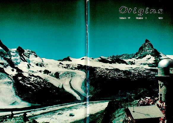
COVER PICTURE. View of the Matterhorn from Gornergrat, Switzerland. It is generally believed that the Matterhorn was formed by the carving action of glaciers. The continuation of the picture on the back cover shows contemporary glacial activity. Several side glaciers are flowing down the Gornergrat glacier found on the floor of the main valley. For further discussion of the time implications of glaciation, see the main article by Michael J. Oard. Photo by Ariel A. Roth.