
Abstract
Biplot diagrams are traditionally used for rock discrimination using geochemical data from samples. However, this approach has limitations when facing a high number of variables. Machine learning has been proposed as an alternative to analyze multivariate data for more than 70 years. However, the application of machine learning by geoscientists is still complicated since there are no tools that propose a pipeline that can be followed from preparing the data to evaluating the models. Automated machine learning aims to face this issue by automating the creation and evaluation of machine learning models. The contribution of this work is twofold. First, we propose a methodology that follows a pipeline for the application of supervised and unsupervised learning to geochemical data. Both methods were applied to a dataset of granitic rock samples from 6 blocks in the Peninsular Ranges and the Transverse Ranges Provinces in Southern California. For supervised learning, the Decision Trees model offered the best values to classify the samples from this region: accuracy: 87%; precision: 89%; recall: 89%; and F-score: 81%. For unsupervised learning, 2 components were related to pressure effects, and another 2 could be related to water effects. As a second contribution, we propose a web application that follows the proposed methodology to analyze geochemical data using automated machine learning. It allows data preparation using techniques such as imputation and upsampling, the application of supervised and unsupervised learning, and the evaluation of the models. All this without the need to program.
Introduction
The application of machine learning in geoscience has a history of around 70 years (Dramsch 2020). Machine learning can be defined as the ability of computers to recognize patterns without being explicitly programmed. Nowadays, different authors have proposed machine learning approaches in remote sensing (Lary et al. 2016), rock classification and predictions (Saporetti et al. 2018), mineral identification (Scott and Steenkamp 2019), and more.
Machine learning can be an alternative to multivariate analysis in geosciences. For instance, although discrimination diagrams have been widely used since 1973 by geoscientists to classify rock samples (Pearce and Cann 1973), they present limitations such as: 1) leaving out important elements of the samples, so the results may be limited; 2) the overlap between the data when plotting; 3) they are effective only for a specific type of rock and even then, they can produce misclassifications; 4) discriminating the same sample with different diagrams can give different results; 5) the samples must meet certain requirements in their composition, even if the diagram indicated for their type is used; and 6) some plots are created with samples from a specific region, so their use cannot be generalized (Li et al. 2015; Armstrong-Altrin and Verma 2005).
Nevertheless, the applicability of machine learning has limitations because it is necessary to have logical reasoning, programming experience, knowledge of algebra, statistics and calculus, and so on (Janakiram 2018). Furthermore, the creation of a highly efficient machine learning model is a time-consuming process, as it involves: cleaning and preparing the data, testing different algorithms, finding the most optimal hyperparameters, and evaluating the models with the appropriate metrics (Vieira et al. 2019).
As a solution, automated machine learning (autoML) is a growing trend to face the complexity of machine learning to end users. AutoML consists of automating machine learning processes to reduce the time to create machine learning models. Also, it allows rapid implementation, and makes machine learning techniques more accessible without advanced programming knowledge (Yao et al. 2018; Hutter et al. 2019).
AutoML platforms such as H2OFootnote 1, DataRobotFootnote 2, and Cloud AutoMLFootnote 3 allow the automatic creation and evaluation of machine learning models. However, they are not free and some may still require prior programming knowledge.
In order to facilitate the application of machine learning to geoscience, our contribution is twofold. First, we present a methodology that follows a simple pipeline, allowing geoscientists to perform machine learning analysis on geochemical data. The methodology consists of: data preparation and analysis with supervised and unsupervised learning. First, the methodology starts with data preparation using techniques such as data imputation and upsampling. Then, supervised learning can be used for classifying samples with 5 classification algorithms: K-Nearest Neighbors, Decision Trees, Support Vector Machines, Logistic Regression, and Multilayer Perceptron. Unsupervised learning can be used for finding patterns with Principal Component Analysis (PCA) and clustering.
Our second contribution is a web application that applies the proposed methodology allowing geoscientists to analyze geochemical data with autoML. This web application does not require programming. The methodology and the web application were used to analyze a dataset of granitic rocks from Southern California using supervised and unsupervised learning.
This paper is organized as follows: “Framework for our approach” presents the framework for our approach. Section “Related work” presents the related work. Section “Methodology” presents the methodology. Section “Web application for AutoML” presents the web application for autoML. Section “Case study” presents the application of our approach to a case study. Finally, “Conclusions and future work” presents the conclusions and future work.
Framework for our approach
Our approach is based on the following concepts (see Fig. 1):

Underpinnings of our approach
-
1.
Machine learning: Machine learning is a branch of artificial intelligence that allows computers to apply different techniques to learn from past experience (Alpaydin 2010). Thanks to machine learning, the computer learns without being explicitly programmed. Machine learning involves different areas such as computer science, engineering, statistics, data mining, and pattern recognition. Its two most used techniques are supervised and unsupervised learning (Harrington 2012; Mohammed et al. 2016). In supervised learning, the data is labeled. A label is a category or class to which the sample belongs to and identifies it. Multiple samples can belong to the same class (have the same label). The algorithms learn from the features of each sample to predict new samples. The features are the measurable properties of the samples. Depending on the feature values (independent variables) it will be the class (dependent variable) to which it belongs. In unsupervised learning, the data is not necessarily labeled. The algorithms group the samples into clusters to discover patterns in them.
-
2.
Automated machine learning: In machine learning, experience is necessary to program, train, and choose algorithms. AutoML automates these steps. Thanks to autoML, machine learning results can be obtained without having advanced technical expertise in the area of programming (Goyal 2019).
-
3.
Supervised learning: The following algorithms are the most commonly used for classification (Osisanwo et al. 2017):
-
(a)
K-Nearest Neighbor: In this algorithm all available cases are stored. New samples are classified based on the most frequent label of its k nearest neighbors (the cases with the data most similar to it) Harrington (2012).
-
(b)
Logistic Regression: This algorithm models the probability of an outcome based on the individual features (independent variables). The features are multiplied by a weight and then added. This sum is put into a logit function, and returns a result that can be taken as a probability estimate (Harrington 2012).
-
(c)
Decision Trees: This algorithm splits the data into subsets (creating a tree) based on the most important features that make the set distinct. It has decision blocks and terminating blocks. In decision blocks, there are 2 alternatives, depending on whether the condition is true or false. They can lead to another decision block or a terminating block. In a terminating block some conclusion has already been reached.
Each block has a measure called entropy. Entropy measures the disorder or uncertainty in a group of samples. The higher the entropy, the messier the data is. The Decision Trees algorithm tries to decrease this measure as each block progresses. When a conclusion is reached (in a terminating block), the entropy is 0 (Harrington 2012).
-
(d)
Support Vector Machines: In this algorithm, the data is plotted in a n-dimensional space (number of features) and a decision boundary (or hyperplane) splits the data into classes. The farther the plotted data points are from the decision boundary, the more confident the algorithm is about the prediction. The data points closest to the hyperplane are called support vectors (Harrington 2012).
-
(e)
Multilayer Perceptron: It is the most common artificial neural network (ANN). It has 2 layers directly connected to the environment (input layer and ouput layer). The intermediate layers between these 2 are called hidden layers. Each layer contains neurons connected to the next layer. The signal transmitted by neurons follows a single direction (from the input layer to the output layer) without forming loops. This structure is called feed forward. It also uses an algorithm called backpropagation to minimize errors between the model outputs and the expected outputs (Marius et al. 2009).
-
(a)
-
4.
Unsupervised learning: Data reduction and clustering are commonly used together in unsupervised learning to improve accuracy by reducing the dimensions of the data (Ding and He 2004). In this research work, the following 2 unsupervised learning methods are used:
-
(a)
PCA: It is a technique used to reduce the dimensionality of the data while losing as little information as possible. The dataset is transformed to a coordinate system. A first axis is chosen in the direction of the most variance in the data. A second axis is chosen orthogonal to the first axis and with the largest variance that it can. This process is repeated until all the data is covered on the generated principal components (PCs) (Harrington 2012).
-
(b)
K-Means: It is an algorithm to form clusters with similar characteristics. The center of each cluster is called centroid, and it is the mean distance of the values in each cluster. The K-Means algorithm finds k unique clusters and each sample is assigned to the cluster with the closest centroid (Harrington 2012).
-
(a)
-
5.
Web Application: A web application is any tool that is hosted on a web server, which is accessed via a web browser. Its functions can be of any type, and can be very simple to very complex. Because it is hosted on a server, it is not necessary to install the application on a computer. Rather, it interacts with the data from the web, creating a client-server environment. Any application used to enter the information is called client. The server can be any hardware or software that uses different protocols to respond to client requests.
Related work
Several authors have proposed the application of machine learning techniques to solve problems in geochemistry. Table 1 summarizes these research works.
Supervised learning
In the following research works, the authors compared several supervised learning approaches to create optimal classifiers and predict new samples.
In Itano et al. (2020), the authors proposed the use of Multinomial Logistic Regression to discriminate the source rock of detrital monazites. They used 16 elements (La, Cr, Pr, Nd, etc.) from samples of detrital monazites from African rivers. All possible combinations were created using the 16 elements (65,535 different combinations) to obtain the models with the best discrimination. Accuracy values by number of elements were compared and the results showed that the highest accuracy (97%) is obtained with 8 to 10 elements.
In Maxwell et al. (2019), the authors applied 3 classification algorithms (Random Forest, Gradient Boosted Machine, and Deep Neural Network) to predict altered and non-altered lithotypes. They used a dataset with geophysical log data from 1,230 coal samples taken from 263 boreholes from the Leichhardt Seam of the Bowen Basin in Eastern Australia. The dataset was randomly splitted into an 80% training set and 20% testing set. The Random Forest model performed the best with average results of: 99% precision, 99% recall, and 99% F-score for the training set; for the testing set: 97% precision, 93% recall, and 95% F-score. Only 11 classifications out of 1,230 samples were identified wrongly.
In Hasterok et al. (2019), the authors compared and discarded different approaches (Discriminant Analysis, Logistic Regression Analysis, Decision Trees, etc.) to develop an accurate protolith classifier. A dataset was created and normalized extracting 9 major elements (SiO2, TiO2, Al2O3, MgO, etc.) from 533,360 samples: 497,401 igneous samples and 35,959 sedimentary samples. The samples were taken from a global dataset of rock major elements. The results showed that the best classifier was an Ensemble Trees model (RUSboost) with an accuracy of 95% true igneous and 85% true sedimentary.
In Ueki et al. (2018), the authors compared 3 classification algorithms (Support Vector Machine, Random Forest, and Sparse Multinomial Regression) for the discrimination of volcanic rocks according to 8 tectonic settings. The dataset was obtained from 2 global geochemical databases: PetDB and GEOROC. It was composed of 24 geochemical data and 5 isotopic ratios (29 features) and contained 2,074 samples. The results showed that the 3 methods presented an accuracy higher than 83% in most of the classes. Although the accuracy of Sparse Multinomial Regression was the lowest, it was the most useful method for generating geochemical signatures that were easy to interpret and analyze.
In Petrelli and Perugini (2016), the authors used Support Vector Machines to classify rock samples according to 8 different tectonic settings. The dataset was composed of major elements, trace elements, and isotopes, from 3,095 samples. They classified the samples using major elements, trace elements and isotopes separately, and the combination of all (4 experiments total). The results showed that the combination of the major elements, trace elements, and isotopic data offers the highest accuracy (93%) than separately: 79% for major elements, 87% for trace elements, and 79% for isotopes.
Unsupervised learning
In the following research works, unsupervised learning was used to find patterns in geochemical data. They also show the relationship between data reduction and clustering.
In Ellefsen and Smith (2016), the authors applied a clustering method based on a hierarchy to interpret geochemical data from the soil of Colorado, USA. The dataset was cleaned based on the concentration percentage of the elements, and PCA. The final dataset contained 959 samples with 22 principal components. The results of the hierarchy method were 2 clusters, each one with elements in common. Cluster 1 contained elements commonly enriched in shales and other fine-grained marine sedimentary rocks. Cluster 2 contained elements commonly associated with potassium feldspars or felsic rocks. The plotted results were consistent with the geological units in the area.
In Jiang et al. (2015), the authors applied PCA and Hierarchical Cluster Analysis (HCA) to study the geochemical processes that control the presence of As in groundwater in the Hetao basin, Mongolia. 90 groundwater samples with 22 geochemical parameters (Ca, Cl, Na, NO3, pH, etc.) were collected from the area. PCA was applied to the samples and they identified 4 major principal components that explain 78.2% of the variance of the original data. The components were the input for the HCA method. The results showed 3 clusters. In Cluster 1, high As concentrations correspond to high P concentrations in flat plain. In Cluster 2, samples are affected by lithological and redox factors. In Cluster 3, low As concentrations correspond to low P concentrations in alluvial fans.
In Alférez et al. (2015), the authors compared PCA and Geographic Information Systems (GIS) techniques with the K-Means clustering algorithm. The authors used geochemical data from 800 rock samples from an area of Southern California. The approaches were compared in terms of 4 geochemical factors: SiO2, Sri, Gd/Yb, and K2O/SiO2. The results showed that the K-Means algorithm gives results very similar to the ones obtained with GIS and PCA.
Discussion
According to the research works presented above, supervised learning is more used than unsupervised learning in geochemistry. In general, research works on supervised learning use the following methodology: cleaning and selecting the data, splitting the dataset, training the algorithms, and showing the results. However, several of these research works lack specific activities for data preparation, such as imputation, removing null values, or sample balancing. Also, they tend to leave out other metrics besides accuracy to evaluate and compare the models. There is no work proposing a machine learning platform or an autoML tool for geochemical analysis.
Methodology
The methodology proposed for applying machine learning to geochemical data is as follows (see Fig. 2).

Pipeline to apply machine learning to geochemical data with autoML
First, the data is entered and prepared using imputation or removing null values. Then, the learning method to be applied is chosen. For supervised learning: 1) the class and features are selected; 2) the user can choose to balance the data or not; 3) the dataset is splitted; 4) the models generated are automatically trained and evaluated; and 5) the best model is used to classify new samples. For unsupervised learning: 1) the features are selected; 2) PCA is applied; and 3) K-Means clustering is applied. These steps are explained as follows.
Data preparation
In this step, the dataset is uploaded and prepared. The user can choose to apply imputation to fill null values. Otherwise, the user can choose to remove samples with null values. Specifically, the following activities are carried out during data preparation:
-
1.
Upload the dataset: The user uploads the dataset to the server. Our web application is publicly available.Footnote 4 First, the file must be in the comma separated values (CSV) format. The CSV format is widely used to store raw data. Each column must be identified with a name. Also, the CSV dataset must only contain numeric or string data values to avoid problems when reading special characters. For example, characters such as <, >, %, or ˆ are not allowed. For supervised learning, samples must be labeled by strings of characters or categorical values (integer natural numbers). For unsupervised learning, it is not necessary to have labeled samples.
-
2.
Apply imputation: If the dataset has samples with missing values, the user can decide to use imputation. If the user decides not to use imputation, then the samples with null values are removed. Imputation refers to filling empty spaces with different values. The web application uses the Extra (extremely randomized) Tree Regressor to perform this technique (Geurts et al. 2006). Extra Tree Regressor is an Ensemble Decision Tree algorithm. It can produce better results than Decision Trees because it splits each node randomly instead of looking for the most optimal split.
Supervised learning
In this step, the classification algorithms are trained and evaluated. The most accurate model is then used to classify new samples of data. The activities to apply the supervised learning method are described as follows:
-
1.
Select the features and the class variables: The features and class variables to train the algorithms are selected. In the web application, the class labels can be string of characters or numeric categories, and the features must be numeric values.
-
2.
Balance the data: The upsampling method can be applied to prevent the most frequent one from dominating the algorithm. Upsampling consists of randomly duplicating samples of the least frequent class until its quantity is the same as the most frequent class. Also, the classes with which the classifiers will be trained are selected.
-
3.
Split the data: The percentage of data used for training is selected and the rest is used for testing. Commonly between 70% and 80% of all data is used to train the models and the rest is used to evaluate their performance.
-
4.
Compare the classification models: The data is finally entered in the classifiers for training and evaluation. The web application uses the HPO (Hyper Parameter Optimization) technique to find the best configuration for each model. A hyper parameter is a defined variable that affects the performance of the algorithm. In HPO, several values for each hyper parameter are selected, and the model is evaluated with the possible combinations (Feurer and Hutter 2019). Then, the model with the best performance is automatically chosen. The following metrics are used to evaluate each model:
-
(a)
Accuracy: It represents the percentage of samples classified correctly out of total samples. It is defined by the following formula:
$$Accuracy = \frac{Correct predictions}{Total predictions}$$ -
(b)
Precision: It represents the percentage of samples correctly identified as positive (true positives) out of total samples identified as positive (true positives + false positives). It is defined by the following formula:
$$Precision = \frac{TP}{TP+FP}$$ -
(c)
Recall: It represents the percentage of samples correctly identified as positive (true positives) out of total positive samples (true positives + false negatives). It is defined by the following formula:
$$Recall = \frac{TP}{TP+FN}$$ -
(d)
F-score: It represents the harmonic mean between precision and recall. It is defined by the following formula:
$$\textit{F-score} =\textit{2 * }\frac{Precision*Recall}{Precision+Recall}$$ -
(e)
Feature importance: It is an additional metric for the Decision Trees classifier. It represents the percentage of how much the model performance decreases when a feature is not available. A feature is important if shuffling its values increases the model error.
-
(a)
-
5.
Predict new samples: In this step, the samples from a new dataset are classified. The new dataset must contain only the features selected in Activity 1 (Select the features).
Unsupervised learning
In this step, the features of the dataset are reduced using the PCA technique. The PCs generated are used as input to the K-Means clustering method. The activities to apply the unsupervised learning method are described as follows:
-
1.
Select the features: The features to be analyzed by PCA and clustering are selected. The features must be continuous numerical values, not categorical. Although PCA can be applied to discrete values, it is not recommended because the variance is less significant in them and the results obtained are less relevant.
-
2.
PCA: The PCA technique is applied for data reduction. It aims to reduce a large number of variables to a (much) smaller number losing as little information as possible. Each component contains the combination of the original variables and the largest variance available in the data. PCA reduces data noise by grouping multivariate into fewer components.
-
3.
K-Means clustering: The PCs that were obtained with PCA are used as input for the K-Means clustering algorithm. Clustering consists of grouping unlabeled samples with similarities between them. The clusters help to understand the organization of the data in a summarized way.
Web application for AutoML
The FlaskFootnote 5 micro framework was used to create the web application for autoML. Flask was chosen in this research work because it provides tools to define routes, manage forms, render templates, etc. while external packages can extend it Grinberg (2014). Flask has two main dependencies: Werkzeug provides the routing, debugging, and Web Server Gateway Interface (WSGI) subsystems; and Jinja2 provides support for the view component. A view is the response sent by the application for a web request and each view is associated with a specific route.
In Flask, the operations with the data are performed by the model components and when finished, it redirects to a view. The view and model components of the web application were programmed in Flask using Python. A Python file contains the definition of the routes, functions, and views of the web application. The interactions between the user and the components in the web application are as follows (see Fig. 3).

Components in Flask of the web application
First, the user enters the web application and the route of the Index() function (see step 1 in Fig. 3) is requested. When the route matches, the function renders an HTML template and displays it to the user (see step 2). The HTML templates contain forms where the user chooses the operations to be applied to the dataset uploaded by the user. In the HTML template, the user enters the dataset to analyze. Once the form is submitted, the path belonging to the Add_CSV() function is requested (see step 3). The Add_CSV() function reads the CSV file and converts it to a dataframe (see step 4). At the end of its operations, the function redirects to the route of the Imputation() function and the process repeats again from step 1 until it reaches an endpoint in the pipeline.
The underlying process followed by the web application is shown in Fig. 4. White blocks are the view functions that render the HTML templates, which are the yellow blocks. Blue blocks are functions that work with the data between each view and at the end, they redirect to the next view. Each set of white, yellow and blue blocks corresponds to an activity of the methodology presented in Section IV.

Underlying process of the autoML web application
The data preparation step is composed of 3 view functions, 3 HTML templates, and 3 work functions. The Add_CSV() function transforms the CSV file to a dataframe; the Add_Imput() function applies imputation to the data or removes the null values according to the user’s response; and the Choose_Learning() function redirects to the next step, depending on the analysis that you want to apply to the dataset.
The supervised learning step is composed of 6 view functions, 6 HTML templates, and 6 work functions. The Add_SupFeats() function keeps only the columns selected by the user; the Add_Balance() function applies upsampling or not according to the user’s response; the Add_Split() function splits the dataset to train and evaluate the 5 algorithms, and chooses the most accurate one; the Add_Report() function redirects to the template to enter the new dataset to be classified; the Add_Classify() function classifies the new samples; and the Add_Results() function downloads a CSV file with the samples and their predicted label.
The unsupervised learning step is composed of 3 view functions, 3 HTML templates, and 3 work functions. The Add_UnsupFeats() function applies PCA to the features selected by the user; the Add_PCA() function groups the components into clusters; and the Add_Results() function allows to download the original samples and their assigned cluster in a CSV file.
A session is used to store user information through requests. This functionality was necessary to avoid data lost at the end of the session. The session object creates a cookie to store the content of the session in a temporary directory on the server. The production WSGI (Web Server Gateway Interface) server WaitressFootnote 6 was used for the deployment of the web application. WSGI is a standard used to establish how the web server communicates with the web application.
Case study
Our approach was evaluated with a compositional dataset from 6 fault-separated blocks in the Peninsular Ranges Province and Transverse Ranges Province. The Peninsular Ranges are a group of mountain ranges, stretching from Southern California to Southern Baja California, Mexico. North of the Peninsular Ranges Province is the east-west Transverse Ranges Province. Around this area, there are several faults that allow the subdivision of the provinces: San Andreas, San Jacinto, Elsinore, Pinto Mountain, and Banning. There are 6 structurally-bounded units or blocks bounded by these faults: San Gabriel, San Bernardino, and Little San Bernardino from Transverse Ranges; and San Jacinto, Perris, and Santa Ana from Peninsular Ranges (Baird and Miesch 1984).
The most important geological feature of the Peninsular Ranges Batholith (PRB) is a batholith-wide separation into western and eastern parts based on geophysical criteria. The older western terrain is more mafic and heterogeneous, and plutons were generally emplaced at a shallower depth with a shallower magma source than those in the east. The magmatism in these provinces records a west to east progression of subduction transitioning from an oceanic to a continental arc setting characterized by numerous individual plutons with compositions ranging from gabbro to tonalite (Hildebrand and Whalen 2014).
The dataset is composed of 514 granitic rock samples (quartz diorites, granodiorites, and quartz monzonites) collected from the study area. This dataset contains 8 major elements (SiO2, Al2O3, Fe2O3, MgO, CaO, Na2O, K2O, and TiO2), 36 trace elements (P2O5, MnO, Sc, V, Cr, Mn, Co, Ni, Cu, Zn, Rb, Sr, Y, Zr, Nb, Mo, Cs, Ba, La, Ce, Pr, Nd, Sm, Eu, Gd, Tb, Dy, Ho, Er, Tm, Yb, Hf, Ta, W, Th, and U), sample id, latitude, longitude, and block (as the class) from the collected samples. This dataset is available online.Footnote 7 Two datasets were created from the original dataset. The first dataset was composed by 90% of the samples per block, and the remaining 10% of the samples were used for the second dataset. The first dataset (462 samples) was splitted again for the training and testing of the models (80% for training and 20% for testing). The labels of the second dataset (52 samples) were removed and the samples were used for prediction. Both datasets were used for supervised learning. The original dataset (514 samples) was used for unsupervised learning. The classes were not used for PCA and clustering. Table 2 shows the number of samples per block for the 3 datasets.
For both analyses, the samples with null values were removed in the data preparation step. Figure 5 shows the workflow of the web application. Each screen shows a form where the user chooses the operations to perform on the dataset. The datasets analyzed during the current study are available online.Footnote 8 The evaluation results, a video demonstration of the web application, and the resulting plot images of the analysis are available as supplementary materials.

Workflow of the web application
Data preparation
Data were prepared by eliminating the rock samples with null values. The activities carried out to prepare the data are as follows:
-
1.
Upload the dataset: Step 1 in Fig. 5 shows the screenshot of the interface to enter the dataset. In this case, the training dataset was uploaded to the web application.
-
2.
Apply imputation: Step 2 in Fig. 5 shows a screenshot of the interface to apply or not apply imputation to the dataset. In this example, imputation was not applied, so samples with null values were removed. After removing null values, the remaining dataset was composed of 432 samples. The remaining samples per class were as follows: San Bernardino: 112 samples; Perris: 97 samples; San Jacinto: 89 samples; Santa Ana: 72 samples; San Gabriel: 41 samples; and Little San Bernardino: 21 samples.
-
3.
Choose the learning method: Step 3 in Fig. 5 shows a screenshot of the interface to select the learning method to be applied to the dataset. Supervised learning was applied first and then unsupervised learning.
Supervised learning
Supervised learning was applied to classify granitic samples according to the 6 blocks of the Peninsular Ranges and Transverse Ranges region: San Gabriel, San Bernardino, Little San Bernardino, San Jacinto, Perris, and Santa Ana. The activities carried out in terms of supervised learning were as follows:
-
1.
Select the features and the class variables: The class column and the feature columns were selected (see step 4 in Fig. 5). The column block was selected as the class. The major and trace elements of the samples (44 out of 48 features) were also selected. The following features were left out: latitude, longitude, and sample id.
-
2.
Balance the data: In this step, the data were balanced (see step 5 in Fig. 5). The class with the highest frequency was San Bernardino with 112 samples, and the lowest Little San Bernardino with 21 samples. Upsampling was applied to balance the frequency of the 6 classes. After applying upsampling, the remaining dataset was composed of 672 samples, 112 samples per class.
-
3.
Split the data: The percentage values to split the dataset were selected (see step 6 in Fig. 5). Specifically, 80% of the samples were selected to train the algorithms and the remaining 20% of the samples were used evaluate the resulting models.
-
4.
Compare the classification models: In this step, the web application returns the metrics of the models (see step 7 in Fig. 5). The model with the best performance in this example was the one generated with the Decision Trees algorithm, with an accuracy of 87%. Its precision, recall, and F-score values were also good in general (see Table 3). The classes that the model classified the best were San Gabriel and Santa Ana, both with 95% in F-score. Contrary, San Bernardino was the class with the lowest recall (68%) and F-score (79%).
The 10 most important features of the Decision Trees model and their values are shown in Table 4. Ni and Sc may be the most important as they are compatible elements and highly concentrated in mafic magmas. La, Sr, Y, and Tb are important because of pressure effects while Cs and K2O are important because they are usually associated with magma depth source (Gromet and Silver 1987).
Figure 6 shows the shortest path to reach a conclusion in the Decision Trees model. It is explained as follows. Each block of the tree contains: its entropy value, its condition and the number of samples that meet it, a one-dimensional array that indicates the score value of each class, and the class with the highest score value. When a new sample is introduced to be classified, it is located in the first block. If the condition is met in the first block (Ni <= 0.006), it goes to the decision block on the left and the sample is classified as San Jacinto. If the condition is met in the second block (Cu <= 0.007), it goes to the left block and the sample is classified as Perris. If the condition is met in the third block (Cs <= 0.001), it goes to the left block and the sample is classified as San Gabriel, and so on until reach a conclusion. If the condition is false in this block, it goes to the right and the sample is finally classified as Perris in the terminating block.
Fig. 6 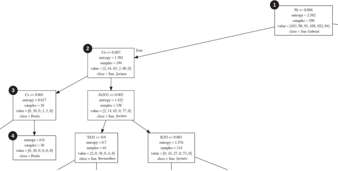
Shortest path to reach a conclusion in the decision tree generated
The accuracy of the remaining models was: K-Nearest Neighbors: 85%; Logistic Regression: 41%; Support Vector Machines: 43%; and Multilayer Perceptron: 77%.
-
5.
Classify new samples: The testing dataset was entered to be classified by the Decision Trees model (see step 8 in Fig. 5). The testing dataset contained the major and trace elements selected by the user. Step 9 in Fig. 5 shows the table with the features and the predicted label for each sample. The table with the sample features and its predicted class can be downloaded in CSV format.

Unsupervised learning
Unsupervised learning was applied to observe the behavior of clusters in terms of geochemical elements. The activities carried out in terms of unsupervised learning were as follows:
-
1.
Select the features: The columns with the features were selected (see step 10 in Fig. 5). The major and trace elements of the samples (44 out of 48 features) were selected. The following features were left out: sample id, latitude, longitude, and block.
-
2.
PCA: PCA was applied to reduce noise in the data and improve the performance of the K-Means algorithm. Step 11 in Fig. 5 shows the screenshot with the table containing the features, and the calculated component loadings. Table 5 shows the eigenvalues, variance percentage, and cumulative variance percentage of the PCs generated. The 5 first PCs were selected to explain 71.9% of the data variance.
-
3.
K-Means: Cluster analysis with K-Means was applied to observe the relationship between the geochemical elements of the samples. Step 12 in Fig. 5 shows a screenshot with the table that contains each sample and its corresponding cluster. The table with the sample features and its assigned cluster can be downloaded in CSV format. According to the Elbow method, 3 was chosen as the optimal value of k (number of clusters). Figure 7 shows the sample clusters plotted by longitude and latitude. The average SiO2 values are as follows: Cluster 1 = felsic @ SiO2 average = 71%; Cluster 2 = intermediate @ SiO2 average = 65%; and Cluster 3 = mafic @ SiO2 average = 58%. However, the average SiO2 values are not quite right to define the compositional groups (for example mafic compositions are not usually higher than 55% SiO2).
The clusters were generated in terms of the samples and geochemical elements. Figure 8 shows the clusters plotted in terms of PC1 and PC2. Positively correlated variables were grouped together (for example: MnO, Mn, and TiO2 are positively correlated). Negatively correlated variables were placed on opposite quadrants of the plot origin (for example: SiO2 is negatively correlated to Fe2O3). The distance between the variables from the plot origin measures the quality of the variables on the factor map (for example: Gd and Dy are more represented in PC2 than in PC1, and Cu and Ni are not well represented in both PCs). PC1 is probably related to compatible/incompatible elements because K2O, SiO2, and Rb were heavily represented on it.
Clusters plotted on PC2 and PC3 show the effects of pressure (see Fig. 9). Sr is positive and Y is negative to PC3 as expected if PC3 is related to pressure. The other Rare Earth Elements (REEs) arrange themselves in between. PC2 does not show much dispersion. However, the large ionic radius elements (K2O and Rb) are negative, and the small ionic radius (MgO, Co, V, and Mn) are positive. For the element clusters: green seems to be heavy REEs (small ionic radius); red are light REEs (large ionic radius); and blue are compatible elements (small ionic radius). For the sample clusters: yellow is high in SiO2, K2O, and Rb (felsic); purple is high in compatible elements (mafic); and green seems to be high in REEs (intermediate).
Clusters plotted on PC4 and PC5 could be related to water effects (see Fig. 10). Immobile Ta and Nb are positive PC4, along with U and Th. For the element clusters: red includes the mobile alkaline elements (Na, K, Rb, and Cs) as well as the immobile ones (Nb and Ta). Perhaps it also includes the elements carried during hydrothermal alteration (Cu, Mo, and W), the radioactive elements (U, Th, K, and Rb) and the Zr-Hf set. For the sample clusters: seem to all center on zero, so the extent of fractionation is not related to water effects. This needs to be studied some more.

Cluster map of the Transverse Ranges Province and the Peninsular Ranges Province in Southern California. The samples were located according to their measured latitude and longitude

Clusters according to PC1 and PC2. For the element clusters: red are large ionic radius, blue are small ionic radius, and green are Rare Earth Elements (REEs)

Clusters according to PC2 and PC3. Large ionic radius (light REEs) and small ionic radius (heavy REEs and compatible elements) are found in element clusters. Felsic, mafic and intermediate elements are found in sample clusters

Clusters according to PC4 and PC5. Mobile alkaline elements and immobile elements are found in element clusters
Discussion
For supervised learning, the Decision Trees algorithm obtained the best average metrics results: accuracy: 87%, precision: 89%; recall: 89%; and F-score: 81%. For unsupervised learning, 5 PCs were used to generate the clusters. The plot with PCs 2 and 3 was found to be related to pressure effects, while the plot with PCs 4 and 5 could be related to water effects.
Conclusions and future work
This research work proposed a methodology to apply machine learning to geochemical data and an open web application for autoML. This tool will allow geoscientists to load geochemical datasets and perform analysis with supervised and unsupervised learning. A dataset composed by granitic rock samples from Southern California was analyzed with both learning methods using the web application. For supervised learning, the Decision Trees model offered the best results. For unsupervised learning, 2 plots were found that could be related to water and pressure effects.
As future work, the proposed pipeline will be extended to apply other techniques to prepare the data, such as downsampling. Also, the web application will incorporate new functions, such as: saving the models created by users to be used more than once, and allowing the tuning of more parameters for supervised and unsupervised learning methods.
Availability of data and material
The datasets analyzed during the current study are available in https://doi.org/10.21227/rcfz-bp27.
Code Availability
The code is not available.
References
Alférez GH, Rodríguez J, Pompe LR, Clausen B (2015) Interpreting the Geochemistry of Southern California Granitic Rocks Using Machine Learning. Proceedings of the 2015 International Conference on Artificial Intelligence (ICAI 2015), Las Vegas, NV, USA
Alpaydin E (2010) Introduction to Machine Learning. MIT press, ch. What is Machine Learning?, pp 1–3
Armstrong-Altrin J, Verma SP (2005) Critical evaluation of six tectonic setting discrimination diagrams using geochemical data of Neogene sediments from known tectonic settings. Sediment Geol 177(1):115–129
Baird AK, Miesch AT (1984) Batholithic rocks of southern california; a model for the petrochemical nature of their source materials. Tech. Rep., reportIt can be improved with the following information in RIS format:TY - RPRT A3 - CY - C6 - ET - - LA - ENGLISH M3 - Report SN - 1284 SP - T2 - Professional Paper VL - AU - Baird, A.K. AU - Miesch, A.T. TI - Batholithic rocks of Southern California; a model for the petrochemical nature of their source materials PY - 1984 DO - 10.3133/pp1284 DB - USGS Publications Warehouse UR - http://pubs.er.usgs.gov/publication/pp1284ER-
Ding C, He X (2004) K-means clustering via principal component analysis. In: Proceedings, Twenty-First international conference on machine learning, ICML 2004, vol 1
Dramsch JS (2020) Chapter one - 70 years of machine learning in geoscience in review. In: Moseley B, Krischer L (eds) Machine Learning in Geosciences, ser. Adv Geophys 61:1–55. Elsevier. http://www.sciencedirect.com/science/article/pii/S0065268720300054
Ellefsen KJ, Smith DB (2016) Manual hierarchical clustering of regional geochemical data using a bayesian finite mixture model. Appl Geochem 75:200–210. http://www.sciencedirect.com/science/article/pii/S0883292716300920
Feurer M, Hutter F (2019) Hyperparameter Optimization.In: Hutter F, Kotthoff L, and Vanschoren J (eds). Automated Machine Learning: Methods, Systems, Challenges.Springer International Publishing Cham. 3–33
Geurts P, Ernst D, Wehenkel L (2006) Extremely randomized trees. Mach Learn 63:3–42
Goyal A (2019) A brief introduction to autoML. https://becominghuman.ai/a-brief-introduction-to-automl-fa6b598d408
Grinberg M (2014) Flask Web development: Developing Web Applications with Python, 1st ed, O’Reilly Media Inc.
Gromet P, Silver LT (1987) REE variations across the peninsular ranges batholith: implications for batholithic petrogenesis and crustal growth in magmatic arcs. J Petrol 28(1):75–125
Harrington P (2012) Machine Learning in Action. Manning
Hasterok D, Gard M, Bishop CMB, Kelsey D (2019) Chemical identification of metamorphic protoliths using machine learning methods. Comput Geosci 132:56–68
Hildebrand RS, Whalen JB (2014) Arc and slab-failure magmatism in cordilleran batholiths II - The cretaceous peninsular ranges batholith of Southern and Baja California. Geosci Can 41:12
Hutter F, Kotthoff L, Vanschoren J (2019) Automated machine learning: methods, systems, challenges. Springer Nature
Itano K, Ueki K, Iizuka T, Kuwatani T (2020) Geochemical discrimination of monazite source rock based on machine learning techniques and multinomial logistic regression analysis. Geosciences 10(2)
Jiang Y, Guo H, Jia Y, Cao Y, Hu C (2015) Principal component analysis and hierarchical cluster analyses of arsenic groundwater geochemistry in the Hetao basin, Inner Mongolia. Geochemistry 75(2):197–205
Lary DJ, Alavi AH, Gandomi AH, Walker AL (2016) Machine learning in geosciences and remote sensing. Geosci Front 7(1):3–10. special Issue: Progress of Machine Learning in Geosciences
Li C, Arndt NT, Tang Q, Ripley EM (2015) Trace element indiscrimination diagrams. Lithos 232:76–83
MSV J (2018) Why do developers find it hard to learn machine learning?. https://www.forbes.com/sites/janakirammsv/2018/01/01/why-do-developers-find-it-hard-to-learn-machine-learning/?sh=d47fe096bf6d
Marius P, Balas V, Perescu-Popescu L, Mastorakis N (2009) Multilayer perceptron and neural networks. WSEAS Transactions on Circuits and Systems, vol 8
Maxwell K, Rajabi M, Esterle J (2019) Automated classification of metamorphosed coal from geophysical log data using supervised machine learning techniques. Int J Coal Geol 214:103284
Mohammed M, Khan M, Bashier E (2017) Machine Learning: Algorithms and Applications. CRC Press
Osisanwo F, Akinsola J, Awodele O, Hinmikaiye J, Olakanmi O, Akinjobi J (2017) Supervised machine learning algorithms: classification and comparison. International Journal of Computer Trends and Technology (IJCTT) 48(3):128–138
Pearce J, Cann J (1973) Tectonic setting of basic volcanic rocks determined using trace element analyses. Earth Planet Sci Lett 19:290–300
Petrelli M, Perugini D (2016) Solving petrological problems through machine learning: the study case of tectonic discrimination using geochemical and isotopic data. Contrib Mineral Petrol 171(10):1–15
Saporetti CM, da Fonseca LG, Pereira E, de Oliveira LC (2018) Machine learning approaches for petrographic classification of carbonatesiliciclastic rocks using well logs and textural information. J Appl Geophys 155:217–225
Scott B, Steenkamp NC (2019) Machine learning in geology. https://www.africanmining.co.za/2019/07/29/machine-learning-in-geology/
Ueki K, Hino H, Kuwatani T (2018) Geochemical discrimination and characteristics of magmatic tectonic settings; a machine learning-based approach. Geochem Geophys Geosyst 19:1327–1347
Vieira S, Garcia-Dias R, Pinaya W (2019) Machine Learning Methods and Applications to Brain Disorders, ch. A step-by-step tutorial on how to build a machine learning model, pp 343–370
Yao Q, Wang M, Escalante HJ, Guyon I, Hu Y, Li Y, Tu W, Yang Q, Yu Y (2018) Taking human out of learning applications: A survey on automated machine learning.arXiv:abs/1810.13306
Acknowledgements
This work has been developed with the support of the Geoscience Research Institute.
Funding
This work was accomplished with financial support of the Geoscience Research Institute
Author information
Authors and Affiliations
Contributions
Credit authorship contribution statement: Germán H. Alférez: Conceptualization, Methodology, Investigation, Writing - original draft, Writing - review & editing, Supervision. Oscar A. Esteban: Investigation, Writing - original draft, Software. Benjamin Clausen: Investigation, Writing - review & editing, Supervision. Ana María Martínez Ardila: Investigation, Writing - review & editing. All authors read and approved the final manuscript.
Corresponding author
Ethics declarations
Conflict of Interests
There are no conflict of interest in this work.
Additional information
Communicated by: H. Babaie
Publisher’s note
Springer Nature remains neutral with regard to jurisdictional claims in published maps and institutional affiliations.
Rights and permissions
Open Access This article is licensed under a Creative Commons Attribution 4.0 International License, which permits use, sharing, adaptation, distribution and reproduction in any medium or format, as long as you give appropriate credit to the original author(s) and the source, provide a link to the Creative Commons licence, and indicate if changes were made. The images or other third party material in this article are included in the article's Creative Commons licence, unless indicated otherwise in a credit line to the material. If material is not included in the article's Creative Commons licence and your intended use is not permitted by statutory regulation or exceeds the permitted use, you will need to obtain permission directly from the copyright holder. To view a copy of this licence, visit http://creativecommons.org/licenses/by/4.0/.
About this article

Cite this article
Alférez, G.H., Esteban, O.A., Clausen, B.L. et al. Automated machine learning pipeline for geochemical analysis. Earth Sci Inform 15, 1683–1698 (2022). https://doi.org/10.1007/s12145-022-00821-8
Received:
Accepted:
Published:
Issue Date:
DOI: https://doi.org/10.1007/s12145-022-00821-8